Sequence assembly

Introduction

Assembly algorithms

Scaffolding

Haplotypes

Assembly quality assesment

Cucurbita example

Human example

Tetraploid potato example

Read cleaning

Having reads of good quality without vector, adaptors, contaminants or chimeras in them is a very important requirement a good assembly. In the CABOG assembler wiki there is a set of recommendations regarding the read pre-processing recommended for different technologies before doing an assembly.

Digital normalization

Recently a paper has been submitted describing and implementing a technique to normalize the coverage, and thus reducing the dataset, before doing a de novo assembly. This algorithm tries to remove reads from over abundant transcripts and it fixes sequencing errors taking into account the low abundant k-mers. Since the assembly is a process very difficult to scale efficiently this could be an interesting approach to ease this problem. This normalization could be of special interest for the transcriptomic assembly. In this case the abundance of the ESTs that correspond to different transcripts differ widely and there is a lot of redundant data for the more expressed transcripts. Given that the requirements of the assembly grow rapidly with the number of reads removing a lot of the redundant reads can simplify the problem a lot.

Some caveats should be considered though. It shouldn’t be used with genomic reads because in this case the highly abundant reads are usually interpreted by the assemblers as repetitive DNA and the normalization would remove this information. This might not be a concern in samples with no repetitive DNA like genomic samples from prokaryotes. Due to the error correction the use of this technique in reads coming from complex samples should also be considered.

The abstract of the paper states the following. Deep shotgun sequencing and analysis of genomes, transcriptomes, amplified single-cell genomes, and metagenomes enable the sensitive investigation of a wide range of biological phenomena. However, it is increasingly difficult to deal with the volume of data emerging from deep short-read sequencers, in part because of random and systematic sampling variation as well as a high sequencing error rate. These challenges have led to the development of entire new classes of short-read mapping tools, as well as new de novo assemblers. Even newer assembly strategies for dealing with transcriptomes, single-cell genomes, and metagenomes have also emerged. Despite these advances, algorithms and compute capacity continue to be challenged by the continued improvements in sequencing technology throughput. We here describe an approach we term digital normalization, a single-pass computational algorithm that discards redundant data and both sampling variation and the number of errors present in deep sequencing data sets. Digital normalization substantially reduces the size of data sets and accordingly decreases the memory and time requirements for de novo sequence assembly, all without significantly impacting content of the generated contigs. In doing so, it converts high random coverage to low systematic coverage. Digital normalization is an effective and efficient approach to normalizing coverage, removing errors, and reducing data set size for shotgun sequencing data sets. It is particularly useful for reducing the compute requirements for de novo sequence assembly.

The authors report that the process requires low memory, works with a single pass and without reference. They also warn that digital normalization should not be used by default if an assembly with all reads can be accomplished.

Practical tasks

Do a manual alignment

Using the inkscape drawing program do a manual alignment of these reads. In any pair of reads a stretch of the same color an letter implies that the reads have a similar sequence in that region. Try to assemble the reads into contigs, but remember that several problems might appear like: repetitive, vector contamination, alternative splicing, etc. Once you have complete the practice you can take a look at the intended result

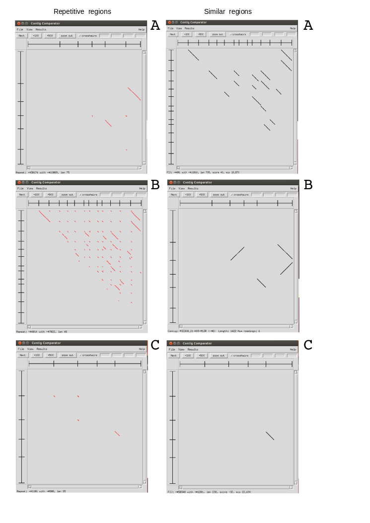
Problems with read cleaning

This is an exercise using Sanger sequences from some ESTs. We have done three assemblies using Staden with different preprocessing filters. To test the results, we have compared all produced contigs between them to identify repeats and very similar regions presents in the contigs of each project. Using this results file, could you identify from which project is each image? Could you explain the results?.

1- Mask regions with Phred quality <15

2- Mask regions with Phred quality <15 and eliminate adaptor and vector sequences

3- Mask regions with Phred quality <25 and eliminate adaptor and vector sequences

Assembly quality assessment

SGN have assembled a draft of the Nicotiana benthamiana genome. The following method was used to do the sequencing. From the DNA, three distinct libraries were synthesized for use in a Illumina HiSeq-2000 sequencer:

• a paired end library with an insert size of approximately 500 bp insert size (4 lanes)

• a mate-pair type library with an insert size of 2kb (1 lane)

• a mate pair with an insert size of 5kb (1 lane)

They show in their web site the summary statistics that correspond to two different assemblies carried out with SOAPdenovo. Which of the two sets of statistics correspond to the v0.3 and v0.42 versions of the assembly? Which one would you prefer?

Statistics that refer to one of the assemblies:

Sequence Count	461,463 sequences
Total Length	2462490758 bp
Longest sequence	208210 bp
Shortest sequence	201 bp
Average length	5336.26 bp
N95 length	1564 bp
N95 index	215459 sequences
N90 length	3403 bp
N90 index	163811 sequences
N75 length	8068 bp
N75 index	96046 sequences
N50 length	16480 bp
N50 index	42984 sequences
N25 length	29264 bp
N25 index	14540 sequences

Statistics for the other assembly.

Sequence Count	3,010,735 sequences
Total Length	2899410662 bp
Longest sequence	103554 bp
Shortest sequence	201 bp
Average length	963.02 bp
N95 length	233 bp
N95 index	2338365 sequences
N90 length	274 bp
N90 index	1763126 sequences
N75 length	619 bp
N75 index	606395 sequences
N50 length	4140 bp
N50 index	156329 sequences
N25 length	10316 bp
N25 index	43823 sequences

Assembler comparison

Several assemblers has been used to assembler the N. benthamiana choroplast (aprox. 100 Kb). The assembly was based on 883811 Illumina pair-ends with a 101 base pairs and and insert size of 400 bp (coverage 1700X). SOAPdenovo was used with all the reads and with a subset. The results of the experiment carried out by Aureliano Bombarely were:

Assembler	Total Scaffold Size (Kb)	Number Scaffolds	Scaffold Max. Len (b)	Scaffold N50	Total Contig Size (Kb)	Number Contigs	Contig Max. Length (b)	Contigs N50	Running Time (min)
SOAP K63 cov >255	1019	7712	1,395	127	1024	7790	547	127	4.75
SOAP K63 subset	134	20	110,468	110,468	133	40	35,718	13,627	0.5
SOAP K63 subset + GapCloser					133	20	109,638	18,725	1
ABySS	170	25	61,293	37,547	170	28	57,534	37,547	20
Velvet					255	1138	2,445	215	2
Ray	1327	10418	45,896	116	1325	10423	45,896	116	20

Which assembler would you use? Would you do any analysis prior to the assembly to make sure that the bulk of the genome is not discarded?

Assembling a mithocondrial genome with SOAPdenovo

We are going to assemble the same 20000 human mithoncondrial pair-end reads with the assembler with a commonly used de brujin based assembler, SOAPdenovo. This assembler only runs on 64-bit operating systems, so if you are using a 32 system you will not be able to run the assembly commands. You can get the final result though and analyze the results.

Create a directory named mito_soap and download and uncompress the reads in it:

~/mito_soap$ pwd
/home/ngs_user/mito_soap
~/mito_soap$ tar -xvzf mito_reads.tar.gz
~/mito_soap$ ls
mito_reads_pe1.fastq.gz  mito_reads_pe2.fastq.gz  mito_reads.tar.gz

SOAPdenovo requires a configuration file to run the assembly. In this file it should be described which are the libraries that are going to be assembled. For each library it should be specified how long are the clone sizes used to create the mate-pairs or the pair ends. If mate-pairs are used it is recommended not to use them during the contig phase, due to the Illumina mate-pairs chimeras (that are usually around 5%), and to reserve them for the scaffolding phase. SOAPdenovo can use the length of the genome to be assembled if this information is known, in this case the human mithodondrial genome has 16.6 kb.

The configuration file would be:

#maximal read length
max_rd_len=101
[LIB]
#average insert size
avg_ins=450
#if sequence needs to be reversed
reverse_seq=0
#in which part(s) the reads are used
asm_flags=3
#use only first 100 bps of each read
rd_len_cutoff=100
#in which order the reads are used while scaffolding
rank=1
# cutoff of pair number for a reliable connection (at least 3 for short insert size)
pair_num_cutoff=3
#minimum aligned length to contigs for a reliable read location (at least 32 for short insert size)
map_len=32
#a pair of fastq file, read 1 file should always be followed by read 2 file
q1=/home/ngs_user/mito_soap/mito_reads_pe1.fastq
q2=/home/ngs_user/mito_soap/mito_reads_pe2.fastq

The command to run SOAPdenovo could be:

~/mito_soap$ soapdenovo2-63mer all -s soap.conf -o assembly -K 35 -p 2 -N 16600 -V
*******************************
 Scaffold number                  6
 In-scaffold contig number        22
 Total scaffold length            13023
 Average scaffold length          2170
 Filled gap number                0
 Longest scaffold                 3046
 Scaffold and singleton number    14
 Scaffold and singleton length    16463
 Average length                   1175
 N50                              2917
 N90                              693
 Weak points                      0
*******************************
Done with 6 scaffolds, 0 gaps finished, 8 gaps overall.

You can download the results and take a look at them.

Usually after running the SOAPdenovo assembler you would also run GapCloser.

Take a look at the assembly kmer frequency distribution. In the file assembly.kmerFreq you can find the number of kmers that were found 1, 2, 3, etc. Does this distribution look OK? What would you expect to find? Which is the expected average coverage given the read length, number of reads and mithocondrial genome length?

Assembling a mithocondrial genome with Velvet

We will use velvet to assemble 20000 human mithoncondrial pair-end reads. Before starting with velvet take a look at its manual.

We will create a directory named mito and we will download the reads in it.

ngs_user@machine:~$ mkdir mito
ngs_user@machine:~$ cd mito/
ngs_user@machine:~/mito$ ls
mito_reads.fastq.gz

velvet is divided in two binaries, velveth and velvetg. velveth creates a hash index and velvetg does the assembly. A critical parameter for the kmer-based assembler is the kmer length. It is usually advisable to run these assemblers with different kmer lengths. In this case we will run velver for 21, 25, 29 and 31. Once we run both commands we obtain the assembly:

ngs_user@machine:~/mito$ velveth  assem 21,31,4 -fastq.gz -shortPaired  mito_reads.fastq.gz
[0.000001] Reading FastQ file mito_reads.fastq.gz
[0.300111] 20000 reads found.
[0.300696] Done
(...)
ngs_user@machine:~/mito$ velvetg assem_21/ -ins_length 500 -exp_cov 30.0 -read_trkg yes -amos_file yes
[0.000001] Reading roadmap file assem//Roadmaps
[0.068547] 20000 roadmaps read
[0.069942] Creating insertion markers
[0.075533] Ordering insertion markers
[0.103541] Counting preNodes
ngs_user@machine:~/mito$ velvetg assem_21/ -ins_length 500 -exp_cov 30.0 -read_trkg yes -amos_file yes
ngs_user@machine:~/mito$ velvetg assem_25/ -ins_length 500 -exp_cov 30.0 -read_trkg yes -amos_file yes
ngs_user@machine:~/mito$ velvetg assem_29/ -ins_length 500 -exp_cov 30.0 -read_trkg yes -amos_file yes

In the assem directories you can find fasta sequences for the contigs in the contigs.fa and the reads assembled into the contigs in the velvet_asm.afg file.

To take a look at the assembly you can use tablet and open the afg file.

Designing a sequencing project

How would you design the sequencing of the Lettuce genome? Genome size: 2.7Gb

Tomato Genome Assembly

The tomato genome was assembled using Roche’s Newbler assembler. Different versions of the assembly were prepared as soon as new data was available.

Version 1.00 (2009-11-27)

Contigs: 118,692 sequences, 762.5 Mb, 50% of assembly in 4,238 contigs of 47,298 bp or longer
Scaffolds: 7,409 sequences, 794.6 Mb, 50% of assembly in 50 scaffolds of 4.5 Mb or longer

Version 1.03 (2010-01-22)

Changes:

• During the assembly we screened for E. coli sequences

• Two new 454 runs (3kb and 20kb) were added to the assembly

Contigs: 110,872 sequences, 762.0 Mb, 50% of assembly in 3,641 contigs of 55,730 bp or longer
Scaffolds: 3,761 sequences, 781.7 Mb, 50% of assembly in 52 scaffolds of 4.4 Mb or longer

Version 1.50 (2010-05-14)

Changes:

• The contigs from assembly 1.03 were polished using the SOLiD data and SOLEXA data. Polishing included single-base error correction and indel correction (mostly homopolymer).

• Contamination from E.coli and vector sequences was removed.

• Several structural inconsistencies were solved.

• Contigs from fully sequences BACs were integrated.

• Superscaffolds were built using clone-end information (BAC and fosmid ends).

Contigs: 29,736 sequences, 733.0 Mb, 50% of assembly in 2,754 contigs of 69,257 bp or longer
Scaffolds: 3,584 sequences, 781.2 Mb, 50% of assembly in 27 scaffolds of 7.8 Mb or longer

Version 2.10 (2010-06-25)

Changes:

• The scaffolds from assembly 1.50 were further linked together by the clone ends (BAC and fosmid)

• The new scaffolds were placed and oriented on the 12 chromosomes by integration of the two physical maps (KeyGene WGP and Arizona SNaPshot), the Kazusa genetic map, and multiple FISH maps.

Contigs: 29,736 sequences, 733.0 Mb, 50% of assembly in 2,754 contigs of 69,257 bp or longer
Scaffolds: 3,433 sequences, 781.3 Mb, 50% of assembly in 17 scaffolds of 16.5 Mb or longer
Pseudomolecules: 12 chromosomes and "chromosome 0", 781.6 Mb

Version 2.30 (2010-08-09)

Changes:

• Sequenced BACs were integrated in the scaffolds of assembly version 2.10.

• After the BAC integration the scaffolds were ordered and oriented on the 12 chromosomes using the two physical maps (Keygene WGP and Arizona SNaPshot), the Kazusa genetic map, and multiple FISH maps.

Contigs: 26,874 sequences, 737.7 Mb, 50% of assembly in 1,996 contigs of 87,129 bp or longer
Scaffolds: 3,232 sequences, 781.4 Mb, 50% of assembly in 17 scaffolds of 16.5 Mb or longer
Pseudomolecules: 12 chromosomes and "chromosome 0", 781.7 Mb.

Which of the steps improved the assembly the most?

Illumina Read correction

We have used bless, an illumina error correction program, to correct our illumina reads. We have calculated the kmer distribution and here you can see the histograms of theses distributions.

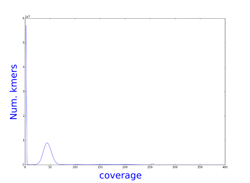
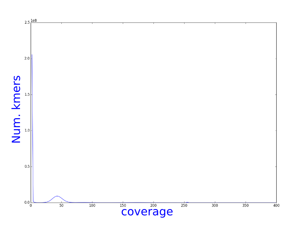
Which one belongs to the corrected reads? Why?

How do you think that this analysis can influence the assembly?